A Step-by-Step Guide for Converting ilumr MRI Scans into STL Meshes for 3D Printing using ITK-SNAP

In the ever-evolving realm of Magnetic Resonance Imaging (MRI), the power of technology has granted us unprecedented insight into the intricate landscapes of organisms, such as, plants and small critters. MRI offers detailed glimpses into the inner workings of their structure, tissues and organs. However, unlocking the full potential of these scans goes beyond mere observation on a 2D screen. With the help of 3D printing we are able to transform these two-dimensional layer snapshots into three-dimensional objects, providing a deeper understanding of their anatomical structures. This can be a useful for educational purposes, as well as, provide a novel opportunity to create oversized models of your favorite small critters and plants.
In this comprehensive guide, we will go through the process Resonint uses to convert MRI scans into immersive 3D models. Whether you're an education provider or an enthusiast seeking visualization tools, this step-by-step guide aims to simplify the process, helping you to breathe life into static images and navigate through the anatomy of the small like never before.
Conversion Guide for 3D MRI data to STL Mesh:
Software Installation
To start the process, install and open your preferred Python integrated development environment (IDE). For this example Anaconda's Spyder IDE was used (https://www.anaconda.com/download).
The other main application required is ITK-Snap (Yushkevich et al., 2006). ITK-Snap is a free, open-source, multi-platform software application used to segment structures in 3D and 4D biomedical images. ITK-Snap can be installed through this link (http://www.itksnap.org/pmwiki/pmwiki.php?n=Downloads.SNAP4).
Acquiring K-Space Data on the ilumr
Open the 3D RARE dashboard on you ilumr desktop MRI system.
Place your selected sample into the ilumr, choose your imaging parameters, and hit the green "Run" button.
Input a workspace name and file name then hit the blue "Save" button. This will save the K-space data from your scan as a .npy file.
Navigate to your workspace on the ilumr (/home/data/<workspace_name>), download the .npy file, and save it to you PC.
Note: If you do not have an ilumr desktop MRI system but still want to follow along with the tutorial, you can download K-space data from our GitHub (https://github.com/Resonint/ilumr-resources/tree/main/kspace_data).

K-Space Data to NIfTI
On you PC, open your Python IDE, navigate to the console and install the nibabel library by typing in "pip install nibabel". Then hit enter.
Create a new python script and copy the code below to convert K-space data to NFiTI format.
Now plug your K-space data's file path into the "numpy_file_path" variable. Then input your desired file output location into the "output_nifti_file_path" variable. Both are located at the bottom of the script.
Run the script.
K-space data to NIfTI code:
import numpy as np
import nibabel as nib


def get_freq_spectrum(signal, dwell_time):
    # returns frequency axis (Hz) and fft (V/kHz)
    N = len(signal)
    fft = np.fft.fftshift(np.fft.fft(signal))
    fft *= dwell_time*1000 # convert to V/kHz
    freq = np.fft.fftshift(np.fft.fftfreq(N, dwell_time))
    return freq, fft


def fft_reconstruction(kdata, gaussian_blur=0, upscale_factor=1):
    # Fourier reconstruction of MRI K-space data

    if len(kdata.shape) == 1:
        tx = np.abs(np.mgrid[-1:1:1j*kdata.shape[0]])
        kdata = kdata * np.exp(-gaussian_blur*gaussian_blur*(tx*tx))
        if upscale_factor > 1.0:
            NX_pad = int((upscale_factor - 1.0)*kdata.shape[0]/2)
            kdata = np.pad(kdata, ((NX_pad,NX_pad)), 'constant')
    elif len(kdata.shape) == 2:
        tx, ty = np.abs(np.mgrid[-1:1:1j*kdata.shape[0],-1:1:1j*kdata.shape[1]])
        kdata = kdata * np.exp(-gaussian_blur*gaussian_blur*(tx*tx+ty*ty))
        if upscale_factor > 1.0:
            NX_pad = int((upscale_factor - 1.0)*kdata.shape[0]/2)
            NY_pad = int((upscale_factor - 1.0)*kdata.shape[1]/2)
            kdata = np.pad(kdata, ((NX_pad,NX_pad), (NY_pad,NY_pad)), 'constant')
    elif len(kdata.shape) == 3:
        tx, ty, tz = np.abs(np.mgrid[-1:1:1j*kdata.shape[0],-1:1:1j*kdata.shape[1],-1:1:1j*kdata.shape[2]])
        kdata = kdata * np.exp(-gaussian_blur*gaussian_blur*(tx*tx+ty*ty+tz*tz))
        if upscale_factor > 1.0:
            NX_pad = int((upscale_factor - 1.0)*kdata.shape[2]/2)
            NY_pad = int((upscale_factor - 1.0)*kdata.shape[1]/2)
            NZ_pad = int((upscale_factor - 1.0)*kdata.shape[0]/2)
            kdata = np.pad(kdata, ((NZ_pad,NZ_pad),(NY_pad,NY_pad),(NX_pad,NX_pad)), 'constant')
    return np.fft.fftshift(np.fft.fftn(np.fft.fftshift(kdata)))


def convert_numpy_to_nifti(numpy_file, output_nifti_file):
    # Load the NumPy file
    numpy_data = np.load(numpy_file)

    # convert kdata to voldata
    blur=1.0 # line broadening/blurring factor
    upscale=2 # zero filling upscaling factor
    voldata = fft_reconstruction(numpy_data, gaussian_blur=blur, upscale_factor=upscale)
    voldata = np.abs(voldata)/np.abs(voldata).max() #normalise

    # Create a NIfTI image
    nifti_image = nib.Nifti1Image(voldata, affine=np.eye(4))

    # Save the NIfTI image to a file
    nib.save(nifti_image, output_nifti_file)


# read file path
numpy_file_path = 'C:/Users/Public/Downloads/Volume Data/Kspace_data/applecore.npy'

# write file path
output_nifti_file_path = 'C:/Users/Public/Downloads/Volume Data/nifti_data/applecore.nii.gz'

# convert numpy file to nifti file
convert_numpy_to_nifti(numpy_file_path, output_nifti_file_path)
NIfTI to STL
Next launch the ITK-Snap application. We will use the saved NIfTI files to produce an STL mesh for your preferred 3D printer model slicer.
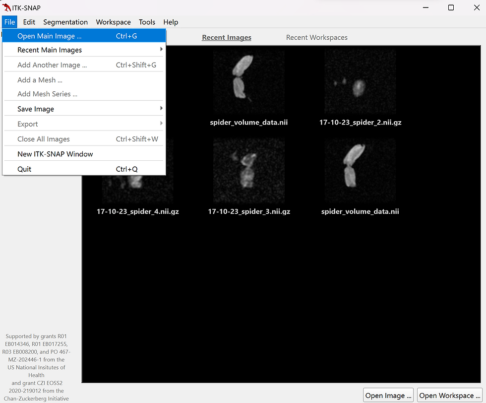
Once the application is open, navigate to the file drop down menu and select open main image (fig.1) or press the Ctrl+G shortcut. Select browse, navigate to your NIfTI file location, and choose your zip file which ends in ".nii".
Once you have selected your NIfTI file, the file format should default to NIfTI. If not, click the file format drop down menu and select NIfTI (fig.2). Hit next and then finish. Now you should see three boxes with different perspectives of your 3D RARE data from the ilumr.
From here, choose the 5th tool from the left of the main tool bar called "Active Contour Segmentation Mode" or press 5 on your keyboard. Red boxes should appear around your MRI slices (fig.3). These boxes define the borders of your data set and create the physical space that your STL mesh will be built in. Use the scroll wheel on each of the three perspectives to find the edges of your image. Scrolling on one perspective will vertically slice through it while the other perspectives mark the layers you are shifting through with blue lines. Click and move the red box walls to match your blue layer lines. Your borders should generally be placed where you can no longer see any white sections in the image (fig.4), unless you intentionally want a cross sectional view.
Now the borders have been defined, select the segment 3D button. Click the drop down arrow in the center the task bar at the bottom of the screen and select continuous update (fig.5). Another option is to press Ctrl+K and then C for the keyboard shortcut.
Next click the "More..." button on the right panel. Here you can choose to display in two different modes in the bottom left. The blue, black and white gradient button makes your three perspectives show what will be excluded from the 3D model in blue. The red and white button with a diagonal line will set the perspectives to show what will be included in your STL mesh in red. for this tutorial we will select the red and white option, but either is perfectly fine. Finally, hit close on that menu.
On the next page you can select your preferred threshold mode. Select lower threshold only (the middle option) and adjust the lower threshold value until the parts of the image you want to model are all red. Avoid decreasing the threshold too far otherwise background noise in the image may also become part of the mesh later on. Scroll through the different perspectives to check over your thresholding. Then, hit next.
Now click and drag the cross hair on each perspective to the center of the main body of your sample and click "add bubble at curser". Next, adjust the bubble radius using the slider so that it doesn't exceed the sample. If there are multiple main bodies, add a bubble to each body. Once you have added all necessary bubbles, hit next.
Press the play button and watch your model grow for over 1000 or so iterations and hit pause when your model starts to slow its growing (fig.6). More iterations aren't always better as this can allows noise to grow into the model. Hit finish.
Finally, select the segmentation drop down menu in the top left and select "export as surface mesh" (fig.7). Type in the file name, select STL mesh in the drop down menu and hit finish(fig.8).
Now you have completed the conversion of your 3D RARE Data to STL mesh, allowing you to 3D print the STL on whatever printer and in whatever material you like!
Figures
References
Paul A. Yushkevich, Joseph Piven, Heather Cody Hazlett, Rachel Gimpel Smith, Sean Ho, James C. Gee, and Guido Gerig. User-guided 3D active contour segmentation of anatomical structures: Significantly improved efficiency and reliability. Neuroimage 2006 Jul 1;31(3):1116-28.


Comments